Stats 101 covers how, when comparing two different groups or people, it’s not enough to simply state what the average differences are. 

We see this in those interminable discussions about who is the GOAT of this or that sport. We can simply compare their average numbers of points, but the NBA now might be scoring more points than the NBA in the 1990s, so while Lebron James may be scoring more points than Michael Jordan, some of that might simply because the NBA is different now (I am fabricating the details out of thin air, much to the horror of my oldest I have no idea nor do I care about the basketball GOAT debate). 

We can kind of get around this by, say, subtracting James’ points from the average for the league in 2025 and subtracting Jordan’s from the same in 1995 and compare the raw numbers. This helps, but it still doesn’t adjust for the distribution. If the NBA league in 2025 has a massive spread—meaning scores swing wildly and being 10 points above average is actually quite common—then James’ lead isn’t that statistically significant. However, if the 1995 league was incredibly tight, where almost everyone scored within 2 points of the average, then Jordan being 10 points ahead makes him a statistical outlier of epic proportions.

To solve this, we can take Jordan’s score in terms of how many standard deviations above the mean he is. Standard deviations is a measure of spread; we don’t need to go into mathematical detail suffice it to say that two standard deviations above and below the average covers about 95% of the scores in the NBA (or times in a race, or IQ scores, or most other things). 

One thing that’s nice about measuring differences by standard deviations is that we can compare very different things on an apples-to-apples basis. It functions as sort of a universal translator for differences. So, with that, in order to really get a sense of how much more religious Latter-day Saints are in a way that takes the background and distribution of religiosity of the US into account, I decided to compare religiosity with a distribution we all sort of intuitively know about: height. If religiosity was height, how tall would Latter-day Saints be? Technical details are in the appendix. 

Conclusion

We’re more religious than average at about the same level that agnostics are less religious than average (about .8 standard deviations above and below the mean, respectively). In height terms, compared to the average man of 5’10, Latter-day Saints are about 6 feet and a half inch if their religiosity was converted to height (while agnostics are about 5’7 and a half).  I also ran these numbers for how religious Utah was compared to other states, and I got .23 standard deviations, or about two thirds of an inch of height. 

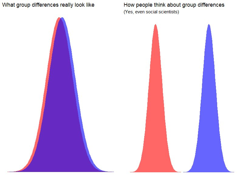
If these don’t sound like large differences to you, and you were expecting Latter-day Saints or Utahns to be NBA stars, religiously speaking, here is a meme I ran across.

---

Technical Details

I drew from (what else) the Cooperative Election Study. Specifically, I subset all of the 2020 years to get a solid Latter-day Saint sample size. I then calculated the weighted mean and weighted standard deviation of the religious attendance measure (inverted, since the directionality originally has more attendance having a lower score for some reason). I then ran a weighted average by group and then generated Z-scores from those averages. 

I then found an estimate for the mean and SD of height of men in the US (I found a couple different estimates that varied slightly, I settled on an average of 5’10 with a SD of 3 inches), and then used that to generate a graph of Z-scores by inch-by-inch (male) height. 

Code

library(haven)
library(pollster)

df <- read_dta(“~/Desktop/dataverse_files/cumulative_2006-2024.dta”)
df<-subset(df, year>2019)
#Weight_cumulative: https://cces.gov.harvard.edu/frequently-asked-questions

attributes(df$religion)
attributes(df$relig_church)
table(df$relig_church)
attributes(df$state)

table(df$relig_church)

df$relig_church[df$relig_church %in% c(7, 8)] <- NA
df$relattend <- 7 – df$relig_church
table(df$relattend)

weighted.mean(df$relattend, df$weight_cumulative, na.rm = TRUE)
wtd.mean(df$relattend, df$weight_cumulative)

library(Hmisc)

sqrt(wtd.var(df$relattend, weights = df$weight_cumulative, na.rm = TRUE))

library(matrixStats)

weightedSd(
x = df$relattend,
w = df$weight_cumulative,
na.rm = TRUE
)

#2.758545 is the mean for relattend
#1.718029 is the SD

library(dplyr)

religdf<-df %>%
group_by(religion) %>%
summarise(
mean_relattend = weighted.mean(relattend, weight_cumulative, na.rm = TRUE)
)

test<-subset(df, religion==3)
wtd.mean(test$relattend, test$weight_cumulative)

attributes(df$religion)

statedf<-df %>%
group_by(state) %>%
summarise(
mean_relattend = weighted.mean(relattend, weight_cumulative, na.rm = TRUE)
)

religdf$ZScore<-(religdf$mean_relattend-2.758545)/1.718029
statedf$ZScore<-(statedf$mean_relattend-2.758545)/1.718029

#Sources for standard deviations for height
#https://distributionofthings.com
#For the US: https://www.maxwachtel.com/blog-1/2020/6/22/statistics-explained-mean-and-standard-deviation
#5’10, 3 inches slightly different numbers, nice round one.

mean_height <- 70 # 5’10” in inches
sd_height <- 3 # standard deviation in inches

heights_in <- seq(from = 60, to = 84, by = 1)

height_z_df <- data.frame(
height_inches = heights_in,
height_feet_inches = paste0(
heights_in %/% 12, “‘”,
heights_in %% 12, ‘”‘
),
z_score = (heights_in – mean_height) / sd_height
)