TLDR: The occasional art missionary to Europe or groundbreaking female doctor notwithstanding, a few years after the “Utah War” we were still pretty much a people of farmers and day-laborers with hardly any middle-class or educated professions.
It’s hard to compare the relative economies of different states and territories in the 19th century, because the relevant income questions weren’t asked until the 20th century. However, one way we can kind of get at this is what is called the Duncan SEI Index, a measure from 1 to 100 which measures the relative prestige and income of different careers. Of course there are issues with using this,* but it’s the worst measure of occupational prestige in the 1860 census except all the other measures (as far as I know). So I ran the averages by state, and interestingly, if we look at all adults over the age of 18, Utah is…third to last (SEI score of 6/100), beaten out by Colorado and New Mexico (both 5/100). This isn’t super surprising since we’re all frontier locations. The highest is Oklahoma (19), so there’s clearly something weird going on with who they’re surveying in Indian Territory at that point, but the next highest is Washington, DC (13), which makes sense.
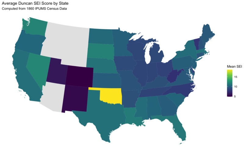
Of course, see caveat in asterisk about indigenous people and slaves, but still, this is evidence that, the occasional art missionary to Europe or groundbreaking female doctor notwithstanding, a few years after the “Utah War” we were still pretty much a people of farmers and day-laborers with hardly any middle-class or educated professions.
- Specifically,
1) The score assignment is based on the prestige of these careers in the 1950s which were then back-applied to the 1860s. So while, say, the prestige and income of a farmer relative to a lawyer has probably shifted somewhat from 1860 to 1950, the order of magnitude is approximately correct, with the doctors, lawyers, and merchants in the higher classes and the farmers and laborers in the lower classes.
2) There has been a metric ton of ink spilled on different SEI index measures and how much they work. This literature isn’t my thing (if you think you’re a heretic because of your political opinions at church, try being a sociology PhD who doesn’t care about inequality research), so I’m just going to appeal to authority with this measure since it’s the most well-known one.
3) I don’t know how this interacts with the indigenous, slaves, and others in (and out of) the census that were certainly not “missing at random” as they say in the data world. As noted, I don’t know why Oklahoma is such an outlier, and there’s clearly something fishy with who the census talked to there.
Code
if (!require(“ipumsr”)) stop(“Reading IPUMS data into R requires the ipumsr package. It can be installed using the following command: install.packages(‘ipumsr’)”)
library(dplyr)
library(tigris)
library(sf)
library(ggplot2)
options(tigris_class = “sf”, tigris_use_cache = TRUE)
setwd(“LOCATION”)
ddi <- read_ipums_ddi(“usa_00032.xml”)
data <- read_ipums_micro(ddi)
data <- subset(data, AGE > 17)
state_means <- data %>%
group_by(STATEFIP) %>%
summarise(
mean_sei = mean(SEI, na.rm = TRUE),
.groups = “drop”
) %>%
mutate(
GEOID = sprintf(“%02d”, as.integer(STATEFIP))
)
state_lookup <- states(cb = TRUE) %>%
st_drop_geometry() %>% # strip geometry, keep attributes
select(GEOID, STUSPS, NAME)
state_means_named <- state_means %>%
left_join(state_lookup, by = “GEOID”) %>%
select(STATEFIP, GEOID, STUSPS, NAME, mean_sei) %>%
arrange(STUSPS)
states_sf <- states(cb = TRUE) %>%
filter(!STUSPS %in% c(“AK”, “HI”, “PR”, “VI”, “GU”, “MP”, “AS”)) %>%
left_join(
state_means %>% select(GEOID, mean_sei),
by = “GEOID”
)
ggplot(states_sf) +
geom_sf(aes(fill = mean_sei), color = NA) +
scale_fill_viridis_c(name = “Mean SEI”, na.value = “grey90”) +
coord_sf(crs = 5070) +
theme_void() +
labs(
title = “Average Duncan SEI Score by State”,
subtitle = “Computed from 1860 IPUMS Census Data”
)
df <- subset(data, STATEFIP == 49)
mean(df$SEI, na.rm = TRUE)
df <- subset(data, STATEFIP == 4)
mean(df$SEI, na.rm = TRUE)
Comments
10 responses to “1860 Utah Had Fewer Skilled and Educated Workers than Almost Any Other State/Territory in the US”
I’d guess that Utah also had fewer pastors per capita, which would have been one of the relatively prestigious professions in small towns and rural areas at the time.
In 1860 there were no art missionaries or groundbreaking female doctors in Utah. Both of those movements came later.
Good points both.
Is Utah now slightly above average in this metric now?
I don’t know, they don’t keep this metric as some kind of year-to-year measure, I’m just using it because it’s the only one available for this time period, but in terms of education level (as measured by holding an undergraduate degree) it looks like Utah is about 13th. https://en.wikipedia.org/wiki/List_of_U.S._states_and_territories_by_educational_attainment. So yes, definitely a bootstraps story from the starvation years to now.
Very interesting! Good piece of research, too. As Rumsfeld would say, we work with the data we have, not the data we’d like to have.
An ancestor of mine was a skilled tradesman when he lived on the east coast back then. Shortly after this census he moved to Utah, but became a farmer because there was little need of his trade in the area where he settled.
After a couple of generations of farmers, none of my generation (descended from the ancestor’s grandson) are farmers now.
Kerry William Bate: Thank you!
el oso: Interesting; yes, I assume a lot of early Utahns were actually skilled and educated, but in the 1860s everybody is just starting to have enough calories to not be constantly thinking about food (and farming) all the time.
Hmm…I’m no economic historian, but I’d expect mean SEI in 1860 to be highest on the east coast, then gradually decrease as you go west with maybe a bit of a bump right on the west coast. Going north to south, my guess is the more industrialized north would be higher than the more agricultural south, but I’m less confident of that. Significantly higher in the south seems unlikely. I’d also expect neighboring states to be fairly similar–big shifts are more likely the result of differences in measurement than reality.
Well, we don’t see that. I’m especially dubious that the region with the lowest mean SEI was the Great Lakes states. On the frontier, I’ll bet there was a lot of undercounting, and it seems plausible that people with higher SEI were more likely to be counted as they were more settled and more likely to be known to the government. (Maybe the reason Utah is so low is that the Church’s networking made the count more complete and thus more accurate.) In the south, I doubt slave occupations were recorded consistently. So I’m kind of dubious about this data anywhere west of the Mississippi or south of the Mason-Dixon line, which is where you get most of the big differences between neighboring states. But Kerry William Bate is right about working with the data we have.
“if you think you’re a heretic because of your political opinions at church, try being a sociology PhD who doesn’t care about inequality research”
Haha, I’ll bet! Just in case any other prospective social scientists are reading though, it seems to me that the evils of economic inequality are a leitmotif of the whole Restoration project. The Nephites may have fallen due to the inward sin of pride, but the outward manifestation of it was inequality. Then there’s the City of Enoch, the United Order, etc. I hope a generation of Latter-day Saint social scientists who remember President Benson’s call to study the Book of Mormon (which has been repeated by subsequent prophets) but forget his politics (which have not) will bring that perspective to the study of inequality.
Not that everyone needs to.
Of course, yes, inequality is important, but so are a lot of other things. My little niche, in-group dig was about the fact that sociologists hardly study anything else in the vast realm of what could be covered by sociology.